
In this article, we continue to explore Big-O, which is a notation we use to describe algorithmic efficiency. If you haven’t read part one, you might like to read that part first.
In the last article we talked about where Big-O notation came from, and what notation we might expect to discover for an efficient or inefficient algorithm. For example the difference between O(1) constant time, and O(N) linear time when looking at time-complexity.
However, now we want to be able to look at an algorithm or a bit of code and work out which Big-O notation for time and space complexity the code or algorithm will start to conform under the conditions of increasing input size. To do this let’s look at one commonly cited example of complexity in algorithms, that is search algorithms.
O(N) Linear Time Algorithms
O(N) refers to where a given operation’s complexity scales linearly with the size of the input. The below algorithm is an example where we want to search for a given string in a given unordered array of strings, we would call this a Linear Search Algorithm, and we could see it for searching for anything comparable in an unordered array.

So, of course, the reason that this is O(N) is that we are taking our worst-case scenario. Whilst the letter we are looking for could be found quickly for a given array, it could equally not be present in the array at all. This means as the size of the input increases, the search time could take proportionally longer (as each checking operation takes the same time per entry in the array).
O(log n) — Logarithmic Time Algorithms
Moving on now to algorithms we can apply to ordered data-sets: Binary Search is an example of algorithm who’s big-O time-complexity will tend towards O(log n) as input size increases. Binary Search also has a O(1) space-complexity, meaning that it doesn’t take up any more memory, no matter the size of the input.
Let’s look at one way to implement Binary Search in Swift using a recursive algorithm (we could alternatively implement this iteratively).

binarySearch Swift
SOURCE: Swift Algorithm Club
Binary Search aims to find the position of a target value within a sorted (or ordered) array (so in the above example it finds 17), and it does this by comparing “the target value to the middle element of the array; if they are unequal, the half in which the target cannot lie is eliminated and the search continues on the remaining half until it is successful. If the search ends with the remaining half being empty, the target is not in the array” (Ref#: D).
Here is a python example:

binary search recursive in python
And here is an illustration of how the search happens for a target of 7 in a sorted array:

sorting image
So we see that binary search tries to get a better search time through a divide & conquer strategy. You can think of a binary search as recursive in nature because it looks to apply the same logic recursively to the smaller and smaller subarrays. To explore then the reason why binary search has a time-complexity of O(log n) we can use Master Theorem for algorithmic analysis, or see the formula worked out here (but intuitively, if we remember that on the graph O(log n) levels out as n increases, we understand that this is because we start to break the problem down into smaller sub-problems which are each faster to solve).
O(n²) — Quadratic Time Algorithms
When we see this notation, we know it is for cases where a given operation’s complexity grows exponentially with the number of inputs (so we want to avoid these if possible). One example of a quadratic-time algorithm is Traversing a 2D array. Another is printing all possible pairs in an array composed of pairs of Ints like:

You can probably see fairly easily here that as soon as we add another pair of integers to our input, we are actually multiplying the number of calculations since we are working out pairs of the x and y between all of the pairs. This means the curve on the graph goes exponential upon adding more inputs.
The Four Rules of Big-O-ifying
Often we may want to work out what the Big-O of a bit of code we are shown is (when we are trying to evaluate what the best solution to a given problem for example). When working out the Big-O of some code, there are four key rules that one should follow when deriving the correct complexity for an algorithm (Ref#: G).
Rule One: Different Steps Get Added
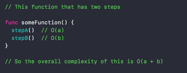
Here a particular function contains two separate processes each of which have their own complexity, these could be the same or different but we will add them together such that with one operation being O(a) and one being O(b) that becomes O(a+b), as above as a first step towards working out the overall complexity.
Rule Two: Drop Constants
So, for example, if you have two operations in a function which both have complexity O(N), then we might naively think that the complexity would be O(2N). However, the collective complexity is not O(2N) as the 2 is not important, we drop the constant therefore and focus on the dominant element in this meaning that indeed the overall complexity is O(N). This also means that if we have a complexity of O(N2 + N2) then that’s just going to become O(N2) since O(N2 + N2) = O(2N2) => O( N2).
Rule Three: Associate Different Inputs with Different Complexity Variables
This rule says that where we have a function taking in two inputs we want to take this into account when we describe the overall efficiency. This is easier to demonstrate with an example:
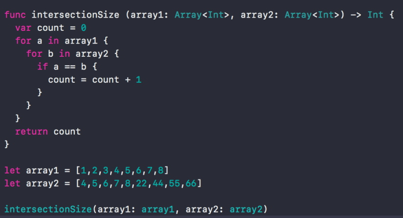
One might intuitively think that the complexity of the above should be described as O(N2), however, this rule suggests, that because we don’t know what N would be describing in this case, but we do know that the length of each of the arrays are factors, then a better way to describe this is as O(a * b), where a is linked to the length of array1 and b to the length of array2.
Rule Four: Drop Non-Dominant Terms
So if you had a function containing an operation of complexity O(N) and another of O(N2) we might be tempted to say that the complexity of the function is something like O(N + N2), but N is going to become less and less important with input size here, it’s basically “non-dominant” so we drop it and, in fact, we just end up with O(N2).
So with these four rules, we should be able to start to think the time and space complexities of a range of different simple algorithms and even novel algorithms, which we are encountering for the first time, and to come up with the correct Big-O notation describing the time-complexity of each. We have also seen in this article some typical examples of algorithms that have a particular time-complexity and the reasons for this. Clearly there are some more complex cases where it can be more challenging to work this out straightforwardly, but the rules for these can also be learnt through more in-depth study of the mathematics involved.
References
A: Know Thy Complexities! (n.d.). Retrieved February 18, 2018, from http://bigocheatsheet.com/
B: Webb-Orenstein, C. (2017, May 11). Complexity and Big-O Notation In Swift – Journey Of One Thousand Apps – Medium. Retrieved February 18, 2018, from https://medium.com/journey-of-one-thousand-apps/complexity-and-big-o-notation-in-swift-478a67ba20e7
C: Hollemans, M. et al. (n.d.). Binary Search. Retrieved February 18, 2018, from https://github.com/raywenderlich/swift-algorithm-club/tree/master/Binary Search
D: https://en.wikipedia.org/wiki/Binary_search_algorithm
E: https://github.com/raywenderlich/swift-algorithm-club/tree/master/Binary%20Search
F: https://en.wikipedia.org/wiki/Master_theorem_(analysis_of_algorithms)
G: https://www.youtube.com/watch?v=v4cd1O4zkGw
H: https://www.youtube.com/watch?v=jUyQqLvg8Qw
Post Updated: 6th May 2018
![]()
Comments