
History of the Notation
Big O Notation is a shared representation (a language if you like) used in computer science to describe how long an algorithm could take to run, and indeed the likely storage or space requirements involved. It “is used to classify algorithms according to how their running time or space requirements grow as the input size grows”. The notation itself belongs to a set of notations which were created by Bachmann, Landau and colleagues and thus given the name Bachmann-Landau notation, or Asymptotic Notation (Ref#: A). The notation was in fact first introduced in Bachmann’s 1892 book “Analytische Zahlentheorie” and it is one of five standard asymptotic notations.

Time-Complexity
The estimate of time taken to run a given algorithm is often called time-complexity. So because we can’t know what future inputs to our algorithm will be, we often choose to take the approach of trying to work out the worst-case time complexity, which is the maximum amount of time taken by the algorithm as when the size of the input gets bigger and bigger. Since this function is generally difficult to compute exactly, and the running time is usually not critical for small input, one focuses commonly on the behavior of the complexity when the input size increases, the behavior of a given algorithm as the input size heads towards infinity that is, and this is called finding the asymptotic upper bound (Ref#: E).

Space-Complexity
Space-Complexity is all about amount of working memory or storage an algorithm is likely to require. We want to know how much memory is going to be used up by a given algorithm during its lifecycle, and similarly to when we looked at time complexity, we want to focus on the wort-case scenario. We can come up with a big-O notation for this worst-case scenario, this represents again what the maximum amount of storage is which our algorithm will use as the input size increases toward infinity.
We can clearly tell from the above that time complexity is not the same as space complexity because they are representations of two different kinds of resource which our algorithm will use, the resource of time, and the resource of memory space.
Disambiguation: whilst in interview Big-O is the most commonly referenced of the notations in technical tests, there is also big-Omega (Ω) which represents the lower bound of complexity, and big-Theta (Θ) which is where an algorithm has both an upper and a lower bound (given particular constant multipliers or n values) and between the upper and lower bounds is a region of all possible complexity values that could result from running the algorithm (above n0 that is), and this region is “tight bound“. In reality, we actually tend to use this notation (Θ) in most cases, only when the bound region is tight bound to the extent our best and worst case are the same, it is our big-Theta (or so-called average case) in fact. (Ref#: F).

Big THETA Graph illustration.
It is notable that the mathematical definition is not always seen in industry where there is sometimes a definition of Big-O to the tightest possible bound instead of just upper bound, so that is something to watch out for. When we are talking about a particular test case for a given algorithm we tend to talk in terms of Best, Worst, and Expected cases, as opposed to referring to Big-Theta and Big-Omega, and these are used to describe the Big-O time for a particular given input cases.
Differentiating Different Big-Os
Lets look as some of the most common examples of this notation which are used to describe the above mentioned properties of particular algorithmic solutions. Here N represents a problem of size N, and c denotes an arbitrary constant.
So for example problem of size N, a constant-time algorithm (which is an algorithm that does not have a complexity dependent on input size) is give then notation O(1), in contrast a linear-time algorithm (which increases linearly in line with input size) is notated O(N), and a quadratic-time algorithm (which becomes exponential as the input size heads toward infinity) is given the designation O(N2). The table below gives a quick reference guide to some of these typical notations.
Table of Big-O Notations
Notation Name
O(1) constant
O(log(n)) logarithmic
O((log(n))c) polylogarithmic
O(n) linear
O(n2) quadratic
O(nc) polynomial
O(cn) exponential
Let have a look at a graphical representation to help those of us with a visual mind understand what these notations are actually telling us:
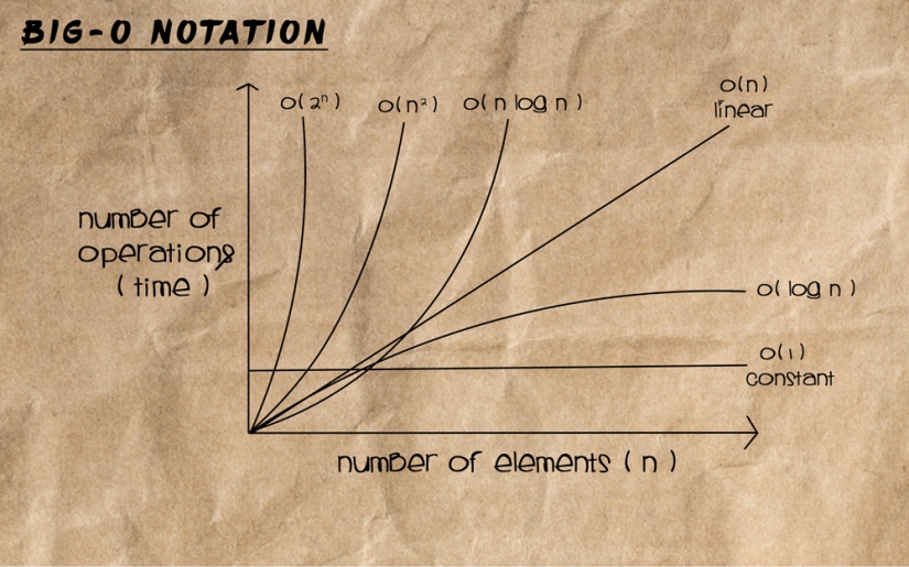
Big O Graph Illustration
From the above graph we can clearly see the Big-O notations we would want the algorithms we use in our code to conform to, are those which don’t end up eating up processor time by becoming increasing inefficient proportional to input size (becoming exponential). We want those where there is either a time to input size static relationship (linear), or which do better and can process larger sets with a better than linear efficiency.
In Part II of this post, we will go through several algorithms for things like search which each have a given Big-O representing their worst-case complexity. We’ll look at how each looks in the Swift programming language, and I will then talk about the efficiency of each, and how we might be able to determine via several important rules-of-thumb that they will conform to particular big-O notation.
References
A: https://en.wikipedia.org/wiki/Big_O_notation
B: https://www2.cs.arizona.edu/classes/cs345/summer14/files/bigO.pdf
C: https://www.interviewcake.com/article/objectivec/big-o-notation-time-and-space-complexity
D: http://web.mit.edu/16.070/www/lecture/big_o.pdf
E: https://en.wikipedia.org/wiki/Time_complexity
F: https://www.cs.northwestern.edu/academics/courses/311/html/space-complexity.html
G: https://www.youtube.com/watch?v=lbLZiHvPIKE
E: https://www.youtube.com/watch?v=v4cd1O4zkGw
F: Mcdowell, G. (2015). Cracking the Coding Interview – 6th Edition. CareerCup, Palo Alto, CA.
![]()
Comments